Tag Archives: algorithms

C++ Implementations of “Engineering the Compiler” Pseudocode

Implementing is understanding

I’m gradually reading through the Engineering a Compiler book. I’m enjoying it but after a while I started wondering if I really understood the algorithms and I wanted to make sure of that before going further. So I implemented the algorithms in C++ (C++17, because it’s nice), testing them against the example inputs and grammars from the book. For instance, here is my code to construct, and use, the action and goto tables which define a DFA for a bottom-up table-driven LR(1) parser, along with some test code to use it with a simple expression grammar.

So far I’ve done this for Chapter 2 (Scanners) and Chapter 3 (Parsers) and I’ll try to keep going. It is a useful exercise for me, and maybe it’s useful to someone else reading the book.  Please note that the code will probably be meaningless to you if you haven’t read the book or something similar. On the other hand, the code will probably seem childlike if you’ve studied compilers properly.

Trying to get  the code to work often showed me that I had had only the illusion of fully understanding. Much of the pseudocode in the book is not very clear, even when you adjust your mind to its vaguely mathematical syntax, and to know what it really means you have to closely read the text descriptions, sometimes finding clues several pages back. For instance it’s not always clear what is meant by a particular symbol, and I found at least one conditional check that appeared in the description but not in the code. I would much rather see descriptions inline in the code.

Pseudocode is vague

I’m not a fan of pseudocode either, though I understand the difficulty in choosing a real programming language for examples. It means putting some readers off. But there could at least be some real code in an appendix. The book has some detailed walkthroughs that show that the authors must have implemented the algorithms somehow, so it’s a shame that I couldn’t just look at that code. I wonder what real programming language might be the most compact for manipulating sets of states when dealing with finite state automata states and grammar symbols.

For the parsers chapter this wasn’t helped by the, presumably traditional, ambiguity of the “FIRST” sets terminology. FIRST(symbol), FIRST(symbols), FIRST(production), and FIRST+(production) are all things.

My code isn’t meant to be efficient. For instance, my LR(1) parser table-building code has some awfully inefficient use of std::set as a key in a std::map. The code is already lengthier than I’d like, so I would prefer not to make it more efficient at the cost of readability. I’ve also probably overdone it with the half-constexpr and vaguely-concepty-generic Grammar classes. But I am tempted by the idea of making these fully constexpr with some kind of constexpr map, and then one day having the compiler build the generated (DFA) tables at compile time, so I wanted to explore that just a little.

But the book is good

Despite my complaints about the presentation of the algorithms, so far I’d still recommend the book. I feel like it’s getting the ideas into my head , it’s not really that bad, and as far as I know there’s nothing better. Of course, given that I haven’t read the alternatives, my recommendation shouldn’t mean much.

Also, these days I always write up my notes as a bigoquiz.com quiz, so here are my quizzable compiler notes so far.

Suffix Tree: Suffix Array and LCP Array, C++

I played a bit more with my C++ Suffix Tree experiment, gradually exploring how Suffix Trees are equivalent to a Suffix Array and its associated LCP Array, allowing us to do anything with Suffix Arrays (and LCP arrays – Longest Common Prefix) that we can do with Suffix Trees, but with less memory (but only by a constant factor) and, I think, more cache-friendly use of memory. This code is still far from suitable for any real use.

Converting between Suffix Trees and Suffix Arrays

I first moved my previous code for Ukkonen’s algorithm from a branch into master, so we can now construct a SuffixTree from a string, in O(n) linear time. Subsequent insert()s still use the naive O(n^2) code. Traditionally, you’d concatenate all your strings with unique separator characters, but I’m trying to avoid that. And, really, I’m just trying to explore the use of the relevant algorithms – it’s a bonus if I can wrap it up into something useful.

I then added a get_suffix_array_and_lcp_array() method to get the Suffix Array and associated LCP Array, in O(n) linear time. This works by doing a lexicographically-ordered depth first search.

Finally, I added a SuffixTree constructor that takes such a Suffix Array and LCP Array to build the suffix tree, again in O(n) linear time. This iterates over the suffixes in the Suffix Array adding a node for each, walking back up the tree to split at the point specified by the LCP array. I kept the path in a stack for that walk up. This constructor let me test that I could use a Suffix Array (and LCP Array) obtained from the SuffixTree to recreate the SuffixTree correctly.

This was based on the ideas I learned from Dan Gusfield’s Fundamentals of Stringology lectures, specifically part 3. Incidentally, his later discussion of the Burrows Wheeler Transform led me to Colt McAnlis’ wonderful Compressor Head series, which far more people should watch.

Towards a usable SuffixArray API.

I’ve already created a SuffixArray class to do much of what the SuffixTree class can do, such as finding matches for a substring. It currently does an O(log(n)) binary search over the suffix array. But this should be possible in O(m) time, where m is the length of the substring, hopefully with far less string comparisons, just as it is possible with a Suffix Array. This can apparently be done with the help of the LCP Array. Hopefully I’ll get to that.

I also want to implement Kärkkäinen & Sanders DC3 algorithm to construct the Suffix Array directly from the string in O(n) linear time. And, if I understand Dan Gusfield’s lecture properly, we can use the Burrows-Wheeler transform to construct the associated LCP Array also in linear time. Hopefully I’ll get to that too.

Suffix Tree, Ukkonen, C++

I’ve been playing with suffix trees recently, in particular trying to get my head around Ukkonen’s algorithm for suffix tree construction. I’ve got the hang of it now after trying out some code and checking it against this excellent video walk through of Ukkonen’s algorithm by Tushar Roy.

Tries, Radix Trees, Suffix Trees

A suffix tree stores every suffix of a string, or of several strings, and makes it easy to find prefixes of those suffixes, in linear O(m) time, where m is the length of the substring. So it lets you find substrings in O(m) time. So it can be used for full text search, and it’s often used for DNA comparison.

A suffix tree is actually a radix tree (also known as a radix trie), with suffixes inserted instead of just the whole string. A radix tree  is itself a compacted trie (also known as a prefix tree).

A trie (pronounced try) is a tree with characters on the edges, letting you discover the whole string as you traverse the edges, staring with the edge from the root for the first character of the string. For instance, this lets you offer text completion if the user gives you the first few correct characters of a word.

A radix tree compacts the Trie by letting each edge have several characters, splitting the edge only when necessary to distinguish different strings. So, while a Trie containing “abc” would have a chain of root->a->b->c, a Radix Tree would have just root->abc. Adding “abd” would change that to root->ab->c, with another for root->ab->d.

A suffix tree, or radix tree, can save space by storing just the start and end indices of its strings instead of the strings themselves. Then each edge has constant size, and the space for the tree is linear O(m), where m is the length of one inserted string. Or maybe you could say its linear O(nk), for n strings of length k, where k is m considered effectively constant.

For the string “banana” a suffix tree would look like this, with both leaf nodes and intermediate end markers marked with *.

root
    banana*
    a*
     na*
       na*
    na*
      na*

We can add a second string in the same suffix tree, associating values with the leaf at the end of each path, letting us know which items have a particular substring. For instance, if I add “banana” (value 0) and “bandana” (value 1) to a suffix tree, I can ask about “ana” and discover that it identifies both items (value 0 and value 1), via the a->n->a path. The tree looks like this:

ban
   ana (0)
   dana (1)
a (0, 1)
 n
  a (0, 1)
   na (0)
  dana (1)
n
 a (0, 1)
  na (0)
 dana (1)
dana (1)

Suffix Tree Construction

The hard part is constructing the suffix tree. When we insert one string of length m, we actually insert m suffixes. If each suffix insertion takes O(m) time, then the whole construction time is at least O(m^2).

Ukkonen’s algorithm reduces this to O(m) by iterating through the string just once from start to end and using the ideas of an implicit “global end”, the “active point” and “suffix links” to jump to wherever the rest of a smaller suffix should be inserted.

Each “phase” deals with one character from the string, in sequence, performing “extensions” within that “phase” to add suffixes that start with that character. This is useful because of the repeating sub-structure of suffix trees – each sub-tree can appear again as part of a smaller suffix.

Global End

Whenever the algorithm adds a node, that’s going to be a leaf node, meaning the edge to the leaf node will have the actual end of the inserted string. So the algorithm assigns a global end to the edge. We increment that end index each time we process the next character, so these edges get longer automatically.

Active point

The active point identifies a point on an edge in the tree by specifying a node, an edge from that node (by specifying a first character), and a length along that edge. Within every “extension”, the algorithm starts looking for the next character at the active point. Sometimes it will find the next character only because an edge got longer automatically when we incremented our global end.

Whenever it finds the next character from that active point, maybe even after stepping across an intermediate node,  it sets that newly-found position as the active point. This is called Rule 3.

Whenever it doesn’t find the next character from that active point, it adds a node, splitting the edge if necessary. This is called Rule 2. Whenever it splits an edge and creates an internal node, it changes the active point to the same character in a smaller edge, and looks again for the same next character. This lets it do the same split in the smaller suffix. It keeps doing this until all the smaller suffixes have been split in the same way.

This example, with the string “banana”, shows the use of the global end and of Rule 3 and Rule 2. It doesn’t show the use of suffix links yet, because it always splits edges from the root. Note that Ukkonen’s algorithm typically appends a special out-of-alphabet “$” character to the string so it can insert leaf nodes.

b: Look from root. Add to root.

b

a: Look from root. Add to root.

b
ba (because we incremented the global end).

n: Look from root. Add to root.

ban (because we incremented the global end).
an (because we incremented the global end).
n

a: Look from root. Find it (“ana”). Set it as the active point.

bana (because we incremented the global end).
ana (because we incremented the global end).
na

n: Look from previously-found “a”, in “_a_na”. Find it. Set it as the active point.

banan (because we incremented the global end).
anan (because we incremented the global end).
nan

a: Look from previously-found “n” in “a_n_an”. Find it. Set it as the active point.

banana (because we incremented the global end).
anana (because we incremented the global end).
nana

$: Look from previously-found “a” in “an_a_na”. Not found, so add an internal node and add the $. Change the active point to same character in a smaller (suffix) edge: “a” in “n_ana”.

banana$ (because we incremented the global end).
ana
   na$ (because we incremented the global end).
   $
nana$

$: Look from “a” in “n_a_na$”. Not found, so add an internal node and the $.
Change the active point to same character in a smaller (suffix) edge: “a” in “_a_na$”.

banana$
ana
   na$
   $
na
  na$
  $

$: Look from “a” in “_a_na$”. Not found, so add an internal node and the $. Change the active point to root.

banana$
a
 na
   na$
   $
 $
na
  na$
  $

$: Look from root.  Add to root.

 banana$
 a
  na
    na$
    $
  $
 na
   na$
   $
 $

Suffix Links

In Rule 2, when the algorithm splits an edge, adding an internal node, if sets a suffix link for that internal node, pointing to root. If it has previously set a suffix link for any other internal node, while looking for the same character (in the same “phase”), it updates the link for that previously-created internal node to point to the new node.

If the active node is not root after adding the internal node, it also changes the active node via the active node’s suffix link, taking us to a previously-created internal node. As before, this lets us jump to the smaller suffix of the same substring, to make the same split there, but suffix links let us do it even when we are not on an edge from root.

We can see this when using “banbadbans” as an example. We reach this point:

a: Look from “n” in “ba->_n_badban$”. Not found, so add an internal node and add the $. Follow the suffix link from the “n” to the “n” in “a->_n_badban$”.

ba
  n
   badban$
   $
  dban$
a
 nbadban$
 dban$
nbadban$
dban$

a: Look from “n” in “a->_n_badban$”. Not found, so add an internal node and add the $. Follow the suffix link from the “n” to the “n” in “_n_badban$”.

ba
  n
   badban$
   $
  dban$
a
 n
  badban$
  $
 dban$
nbadban$
dban$

a: Look from “n” in “_n_badban$”. Not found, so add an internal node and add the $. Follow the suffix link from the “n” to root.

ba
  n
   badban$
   $
  dban$
a
 n
  badban$
  $
 dban$
n
 badban$
 $
dban$

a: Look from root. Not found. Add to root.

ba
  n
   badban$
   $
  dban$
a
 n
  badban$
  $
 dban$
n
 badban$
 $
dban$
$

Example Code

Here is some example C++ code. It’s also in github, with far more comments.

const auto key_start = key.start_;
const auto key_end = str_end(key);

ActivePoint active;
active.node = &root_;
active.edge_valid = false; // Instead of -1.
active.length = 0;

std::size_t remaining = 0;
auto end_ptr = std::make_shared<KeyIterator>(key_start);
KeyIterator& end = *end_ptr;

// The "phases"
for (auto i = key_start; i != key_end; ++i) {
  ++remaining;
  ++end;

  Node* prev_created_internal_node = nullptr;

  // The "extensions".
  while(remaining) {
    const auto edge_match = (active.edge_valid && active.length) ?
      find_partial_edge(active, i) :
      find_partial_edge(active.node, i);
    const auto edge = edge_match.edge_;
    const auto part_len_used = edge_match.edge_part_used_;

    if (!edge_match.char_found_) {
      KeyInternal prefix(i, end_ptr);

      // Rule 2 extension: There is no match:
      if (part_len_used == 0) {
        active.node->append_node(prefix, value);
      } else {
        auto extra_node = edge->split(part_len_used);
        extra_node->append_node(prefix, value);
        extra_node->suffix_link_ = &root_;

        if (prev_created_internal_node) {
          prev_created_internal_node->suffix_link_ = extra_node;
        }
        prev_created_internal_node = extra_node;

        if (active.node != &root_) {
          active.node = active.node->suffix_link_;
        } else {
          --active.length;
          ++active.edge;
        }
      }

      --remaining;
      continue;
    }

    // Rule 3 extension:
    active.node = edge_match.parent_node_;
    active.edge = edge->part_.start_;
    active.edge_valid = true;
    active.length = part_len_used;

    break;
  }
}

Generic Suffix Tree in C++

However, the basic Ukkonen’s algorithm just stores one string. Before trying Ukkonen’s algorithm, I wrote a templated C++ suffix tree that can contain multiple strings (see the test code), with a simple O(m^2), or possibly O(m^3) construction time.

I created a version that uses Ukkonen’s algorithm, reducing construction to O(m) time, but it doesn’t support multiple inserts. In this implementation, I’ve avoided the need for extra “$” leaf nodes. I’ve also stored the suffix links in a hash table, to avoid wasting space per node even after construction, though that replaces a true constant-time read/write with an amortized constant time hash table insert/lookup.

I’m trying to adapt the Ukkonen-based suffix tree to support multiple inserts. Usually, to create such a “generalized” suffix tree with Ukkonen’s algorithm, you concatenate the strings together, separated by unique out-of-alphabet characters (“$”, “#”, etc), insert the whole thing, then prune the paths you don’t need, but I’d like to avoid that.

I’m not suggesting that anyone use this code for serious work. For now, it’s littered with asserts() and debug output and it’s in need of optimization because it’s generalized for any standard C++ container, such as std::string. For instance, it doesn’t seem wise to store std::string::iterators, instead of pointers, for the start/end ranges on edges. I’m also bothered by the use of std::shared_pointer<>s to share the “global end”, which still take space per edge even after construction.

Alternative Algorithms

Update: I’ve just watched Erik Demaine’s 2012 MIT “Strings” lecture about suffix trees (I needed to watch his previous “Static Strings” lecture first). He doesn’t mention Ukkonen’s algorithm, but does mention a “DC3 (Difference Cover 3)” algorithm by Kärkkäinen-Sanders-Burkhardt (at least the lecture’s student notes call it that) for building suffix arrays in linear time. He shows that a suffix tree can then be constructed from a  suffix array by using the LCP (Longest Common Prefix) of the suffix array to build a cartesian tree, again in linear time. So the whole suffix array construction would be linear time. Suffix arrays themselves anyway offer better data locality than suffix trees and this DC3 algorithm apparently allows parallelization. I hope I find time to explore all that sometime in code.

He also mentions the use of a “suffix tray” to store the edges in each node, to get  O(P  + lg(Σ))) query time, much the same as the O(P) time you’d get with an array, while reducing the overall space complexity to O(T) instead of O(TΣ ). Here P is the size of the query string, T is the size of the text being searched, and Σ is the size of the alphabet. He also mentioned instead using a combination of hash tables and van Emde Boas trees to get O(P + lglg(Σ)) query time. Those parts of the lecture felt quite rushed to me, so I’d like to investigate that sometime too if I find time.
Big-O Quiz: Graph Theory

I’ve been studying more graph theory recently. To take notes that I might remember, I added a Graphs quiz to my Big-O Quiz site. It covers the graph theory mentioned in The Algorithm Design Manual and in the Stanford/Coursera “Algorithms: Design and Analysis Parts 1 & 2“  courses by Tim Roughgarden. I’m adding to it as I work through Tim Roughgarden’s follow-up “Second course in Algorithms“.

It’s often a slightly silly quiz, offering you algorithm descriptions that make no sense for the question’s problem, along with the correct one, but the aim is to just to reinforce my memory by exercising my memory. So I’ve tried to use concise descriptions of problems and algorithms, without trying to be exhaustively correct.

BigOQuiz: C++ Standard Library Algorithms

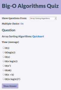
I’ve reworked bigoquiz.com, which I created a few weeks ago. to allow multiple quizzes instead of just the default quiz about the Big-O complexity of algorithms and data structures. For some quizzes it also now offers reversed questions, asking you for the question that matches the answer.

For instance, there is now a C++ Standard Algorithms quiz. You could, for instance, check that you know the descriptions of the Sort Operations functions. Or you could check that you know the names of those Sort Operations functions based on their descriptions (or as multiple-choice). Maybe this is one way to get more familiar with the many standard C++ algorithms that we often don’t realize are available. I hope this helps me as I strive to use “no raw loops“.

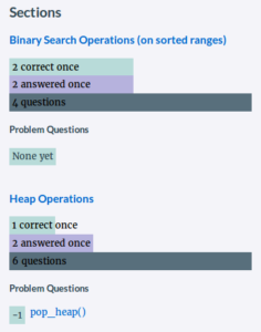
As before, you can track your progress in each section of the quiz, and identify problem questions that you keep getting wrong.

screenshot_bigoquiz_cpp_std_algorithms_sections

I’ve also added a Design Patterns quiz, based on the patterns mentioned in the Head-First Design Patterns book.

The user profile page also now shows overall statistics for all the quizzes that you’ve tried.

screenshot_bigoquiz_userprofile


Playing with C++ Variadic Templates and Dynamic Programming

Dynamic Programming C++ base classes

Over the last few months I’ve been exploring various dynamic programming (DP) algorithms, trying to get a feel for how to choose suitable sub-problems and the dimensions of those sub-problems, and when a top-down or bottom-up strategy is best. In principle, dynamic programming lets you break a problem down into suitable sub-problems, as long as they obey the “principle of optimality“, meaning you can use some broad state (result) of the sub-problem calculation, without needing the actual specifics of each solution.

I’ve also been playing lots with variadic templates in modern C++.

My little murrayc-dp-algorithms project is the result. It has base classes for both bottom-up DP and top-down DP and several examples that use them. The end result is only slightly useful, and is currently far from optimal for performance. But I still think it’s an interesting exercise that shows how these various DP algorithms really relate to each other. It should also explain how I came up with those examples in my earlier blog post.

Top-Down DP

Let’s start with top-down dynamic-programming, because it’s generally simpler. Calculating Fibonacci numbers is the classic example. This is clearly inefficient because every recursive call recalculates almost the same lesser Fibonacci numbers, twice. This is exponential, with time complexity of roughly O(2^n).

int f(int i) {
  if (n == 0)
    return 0;
  else if (n == 1)
    return 1;

  return f(i - 1) + f(i -2);
}

One simple way to avoid the wasteful recalculation is to cache the results and reuse them. That’s generally called Memoization. For Fibonacci number calculation, this is still not the best way, but it’s a useful example.

DpTopDownBase provides a framework for dynamic programming with memoization. You provide a calc_subproblem() implementation, which should use get_subproblem(). That get_subproblem() will return a previously-calculated result if it exists, or recursively call calc_subproblem().

1-Dimensional Top-Down DP

For instance, the top-down DpFibonacci class is declared like so, deriving from DpTopDownBase:

class DpFibonacci
  : public murraycdp::DpTopDownBase< unsigned long, // subproblem type unsigned int // i > {
public:
  explicit DpFibonacci(unsigned int n)
  : n_(n) {}

This specifies that its calc_subproblem() (and the base class’ get_subproblem())will take an unsigned int and return an unsigned long:

unsigned long
calc_subproblem(
  type_base::type_level level,
  unsigned int i) const override {
  // Base cases:
  if (i == 0) {
    return 0;
  } else if (i == 1) {
    return 1;
  }

  return get_subproblem(level, i - 1)
    + get_subproblem(level, i - 2);
}

The level parameter is just for optional debug output, to show how deep we are in the recursive call stack.

It also implements get_goal_cell() so that the base class knows which value of n to use to get the result f(n). This just returns the n provided to DpFibonacci’s constructor.

We can then instantiate the class and call calc():

DpFibonacci dp(n);
auto result = dp.calc();

The base DpTopDownBase::calc() method calls get_goal_cell() and calls calc_subproblem() for that cell. Because our calc_subproblem() implementation uses get_subproblem(), it will automatically avoid recalculating already-calculated sub-problems.

That DpTopDownBase::calc() method is a fairly simple example of the usefulness of C++ variadic template parameters to call one variadic method with the result of another variadic method, using tuples and std::experimental::apply(). And it’s type-safe at compile time all the way.

2-Dimensional Top-Down DP

But DpTopDownBase isn’t just good for a 1-dimensional cache, based on one parameter. The wonder of C++ variadic templates lets us specify multiple parameters for calc_subproblem and get_goal_cell(). Those overridden methods take just the right parameter types and just the right number of parameters.

And this is where top-down DP can be useful, because it might not be necessary to calculate all possible sub-problems for all possible values of these parameters.

For instance, in the Knapsack Problem, we have a knapsack with a certain maximum weight capacity, and we have several items of various weights and values. We want to find the set of items to put in the knapsack that maximises the value. We give each item an index number.

In the classic Knapsack DP algorithm, we then have 2 dimensions (or parameters) for each sub-problem: A count of items and a maximum weight. So if we have 5 items and total capacity of 100Kg, we can calculate the max value, f(5, 100Kg) by using other sub-problems such as f(4, 80Kg) along the way. It’s not likely that we’ll need to calculate all 5 * 100 possible subproblems, though it is likely that we’ll reuse some sub-problem calculations.

For instance, the top-down DpKnapsack class derives from the base DpTopDownBase like so:

class DpKnapsack
: public murraycdp::DpTopDownBase<
    SubSolution,
    SubSolution::type_vec_items::size_type,
    Item::type_weight
  > {

Again it overrides calc_subproblem() and overrides get_goal_cell(). This time it takes 2 parameters instead of just i:

SubSolution
calc_subproblem(
  type_level level,
  type_size items_count,
  type_weight weight_capacity) const override {

And it can call get_subproblem() with those 2 parameters, letting the base class worry about how to cache the sub-problems and when to recalculate them. (This currently uses a rather inefficient generic hashing function for std::tuple<>s. )

Notice that we return a custom SubSolution class for the sub-problem result instead of just a number. This lets us store both the maximum value for that sub-problem and the items used in that sub-problem solution. That helps us to reconstruct the complete set of items for the sub-solutions along the way. However, that is inefficient because we won’t need all sub-solution item sets . It should instead be possible to write some generic code to  reconstruct the solution by working backwards from the result of the goal. I’ll try that out sometime.

Again we can just instantiate the class and call calc():

//Items with their values and weights:
DpKnapsack::type_vec_items items{
  {13, 15}, {12, 14}, {2, 13}, {10, 12},
  {1, 11}, {7, 10}, {6, 9}, {5, 8},
  {11, 7}, {14, 6}, {9, 5}, {4, 4}, {3, 3},
  {22, 2}, {8, 1}};
DpKnapsack::type_value weight_capacity = 45;

DpKnapsack dp(items, weight_capacity);
const auto result = dp.calc();
std::cout << "solution: value: " << result.value << std::endl
  << "with items: ";
print_vec(result.solution);
std::cout << std::endl;

The top-down DpContextFreeGrammarParser , top-down DpMakeChange , top-down DpEditDistance , top-down DpParenthesization do much the same thing. The top-down DpTsp uses 3 dimensions and overrides calc() to choose the minimum result over all the sub-problems at the top level instead of just letting the default base calc() use the result of one goal sub-problem as the overall result.

I think it’s nice to separate the real heart of each DP algorithm from the code that does the boring caching and checking.

Bottom-Up DP

In bottom-up DP, we calculate every single possible sub-problem result, starting from our base case. Even if we won’t need every single possible result, this is often more efficient because we sometimes know when we can discard whole sets of sub-problems. For instance, looking again at the classic Fibonacci Numbers example, we only really need the last 2 sub-problem results:

int f(int n) {
  if (n == 0)
    return 0;
  else if (n == 1)
    return 1;

  int result = 0;
  int prev1 = 1; // f(1) = 0;
  int prev2 = 0; // f(0) = 0;
  for (int i = 1; i < n; ++i) {
    result = (prev1 + prev2);
    prev2 = prev1;
    prev1 = result;
  }

  return result;
}

So we don’t need to cache all i results along the way. For a multi-dimensional DP algorithm, that can save us a lot of space.

1-Dimensional Bottom-Up DP

The bottom-up DpFibonacci class derives from DpBottomUpBase, specifying:

  • the number of sub-problems to keep along the way: 2 to keep f(n-1) and f(n-2).
  • the type of each sub-problem’s (and the final) calculation result: long for the result of f(5), for instance.
  • the type of the input: int for 5, for instance, in f(5).
class DpFibonacci
: public murraycdp::DpBottomUpBase<
    2, // count of sub-problems to keep
    unsigned long, // sub problem type
    unsigned int // i
  > {

DpFibonacci again overrides calc_subproblem() and get_goal_cell(), with exactly the same implementation as the top-down version.

The base class’ calc() method then just iterates from 0 to n, calling the virtual calc_subproblem() method and then returning the result for the goal cell, based on calling the virtual get_goal_cell() method.

DpBottomUpBase keeps just the right number of previously-calculated sub-problems, while reusing the discarded sub-problem storage, by using my (funky) circular_vector.

DpTripleStep is very similar, though it needs to keep the 4 previous sub-problems instead of 2, and of course it does a different calculation per sub-problem.

2-Dimensional Bottom-Up DP

The bottom-up DpKnapsack class is again much like the top-down DpKnapsack implementation, but it again specifies that it only needs the previous 2 sets of sub-problems.

class DpKnapsack
  : public murraycdp::DpBottomUpBase<
    2, // count of sub-problems to keep.
    SubSolution,
    SubSolution::type_vec_items::size_type,
    Item::type_weight
  > {

Where the bottom-up DpFibonacci passed one count to the base class’ constructor, the bottom-up DpKnapsack passes two, one for each calc_subproblem() parameter:

DpKnapsack(
  const type_vec_items& items,
  type_weight weight_capacity)
  : DpBottomUpBase(
      items.size() + 1,
      weight_capacity + 1),
    items_(items),
    weight_capacity_(weight_capacity) {}

The base DpBottomUpBase class uses these constructor parameters as ends of ranges, assuming that each range starts at 0. It will then iterate over the first range, iterating over the second range each time, like a nested for loop:

for (int items_count = 0; items_count < MAX_ITEMS; ++items_count) {
  for (int weight_capacity = 0; weight_capacity < MAX_WEIGHT_CAPACITY; ++ weight_capacity) {
    ...
}

There is no way in C++ to nest an arbitrary number of for loops. But we can use variadic templates to declare an arbitrarily-nested vector. And thanks to my funky variadic templates for vectors of vector (of vectors of vectors, etc), the base class can generically call calc_subproblem() as if it had nested for loops, regardless of how much nesting there should be. My for_vector_of_vectors() takes the (nested) vector, and a series of start and end parameters for each level and eventually uses std::experimental::apply() to call the functor (a lambda, in this case) for each combination. To get that series of start and end parameters, it uses my funky tuple_interlace() to alternate starts (0) with ends.

The bottom-up DpEditDistance and bottom-up DpSubstringMatching do much the same thing.

Problems with DpBottomUpBase

The bottom-up base class has some serious limitations:

It only lets us discard older sub-problems in the first dimension, such as the Knapsack sub-problems for items less than n-2. But you might understand enough about your algorithm to know other sets of sub-problems that can be discarded at various times, based on less simple criteria. This would make the best use of space while avoiding recalculation. Maybe some recalculation would be OK as long as you could minimize it.

Also, it is limited to a simple iteration, using a range from start to end, using a simple operator++ to move to the next iteration. But sometimes you want to do something a little more complicated than an iterating for loop. For instance, my top-down DpTsp class finds a solution for the Travelling Salesman Problem by manipulating sub-sets in its calc_subproblem(). I could use gosper’s hack to create a suitable n-choose-k subset iterator, but it still needs to iterate over a further set of subsets missing each item from the parent subset, and I suppose that would be doable with another custom iterator. But the start and end iterators at each level would then have to be instantiated based on the values of the parent level, and cannot just be supplied before the whole calc() starts. Maybe I could do something with lambda functions to let these iterators be instantiated along the way.

Big-O Quiz: An experiment with Google AppEngine

bigoquiz.com

screenshot_bigoquiz_webOver the last few weeks I’ve been working on bigoquiz.com. I wanted to learn the Big-O algorithmic complexity of the main algorithms and data structures by heart. So, of course, I first built a system to help me do that.

bigocheatsheet.com and bigoref.com already do a good job of listing the information, but bigoquiz.com lets you check that you really know each one, and shows you the ones you keep getting wrong.

Tech I learned along the way

I find it very hard to resist a project when I see that it would let me play with multiple new things. This one was a chance to learn about:

Details

I noticed that bigoref.com had some corrections and additions compared to bigcheatsheet.com. And I made some additions of my own. I’ve listed it all here for anybody who is interested:

For instance,  bigoref.com adds Graph Search algorithms such as Dijkstra’s and Bellman-Ford (missing from bigocheatsheet.com), under “Searching“. I instead listed the graph search algorithms in bigoquiz.com under “Graph Search”  and added more graph algorithms that I’d learned about recently in my Coursera course, though I’m tempted to create a completely different graph algorithms quiz: Kruskal’s Minimum Spanning Tree, Prim’s Minimum Spanning Tree, Floyd Warshall All Pairs Shortest Path, and Johnson’s All Pairs Shortest Path.

bigoref.com also adds linear and binary search of arrays (missing from bigocheatsheet.com). For bigoquiz.com I just split Array into sorted and unsorted in “Data Structure Operations”.

I found just one error on bigoquiz.com that was corrected on bigoref.com, though there might be others:

And I noticed that bigoref.com has some additional errors so I corrected those on bigoquiz.com and  filed github issues for bigoref:

Also:

  • bigocheatsheet.com has entries for Stack, but bigoref.com does not. I kept that in bigoquiz.com.
  • bigoref.com has entries for Ternary Search Tree, apparently a kind of Trie (Prefix Tree), but bigocheatsheet.com does not. I kept this in bigoquiz.com. Curiously, bigoref.com doesn’t have entries for regular Tries (Prefix Trees), or Suffix Trees. I added them to bigoquiz.com, though I’m not completely sure about the various best/worst/average time/space complexities.
  • bigoref.com uses the term “indexing” where bigocheatsheet.com uses “access”. I’ve stuck with “access” for bigoquiz.com.
  • bigoref.com splits array into Basic Array and Dynamic Array, not allowing insertion or deletion in a Basic Array. I don’t find the distinction useful, so I kept it as just Array in bigoquiz.com.

Coursera/Stanford course: Algorithms: Design and Analysis, Part 2

A few weeks ago I mentioned completing Part 1 of the online Coursera/Stanford “Algorithms: Design and Analysis” course. Part 2 of Algorithms: Design and Analysis isn’t due to start again until next year, but I didn’t want to wait, so I enrolled in the archived version of the course to watch the videos and do the assignments. I should be ready to just reuse my work when Part 2 starts again for real.

Part 2 was where things got really interesting. The assignments required implementing these algorithms, though the course covered others too:

  • A Greedy Algorithm for job scheduling.
  • Prim’s and Kruskal’s minimum spanning tree algorithms. (Both O(m log n) but Prims does better on dense graphs, with more edges.)
  • Modifying a minimum spanning tree to identify clusters.
  • The Knapsack problem (Dynamic Programming – both bottom-up and recursive).
  • Shortest Path with the Belmann-Ford SSSP (Single-Source Shortest Path) algorithm (O(mn) and works with negative paths, but fails with negative cycles) as an alternative to Dijkstra’s Shortest Path algorithm (O(m log n) and works only with positive paths).
  • All Pairs Shortest Path with the Floyd Warshall algorithm (dynamic programming) (O(n3) and works with negative paths, though it fails when it detects negative cycles). Best for dense graphs.
  • All Pairs Shortest path with Johnson’s algorithm, via one call to Belmann-Ford on a modified graph and repeated calls to Dijkstra on a reweighted graph. (O(mn log n) and works with negative paths, but fails with negative cycles.) Best for sparse graphs.
  • A dynamic programming algorithm for the Traveling Salesman Problem.
  • Local search with the 2Sat problem, using Papadimitriou’s Algorithm.

I particularly enjoyed exploring “dynamic programming”, which is really just avoiding unnecessary repeated work after you’ve identified the appropriate sub-problems. It’s identifying the sub problems that is really hard. I enjoyed playing with bottom-up dynamic programming (filling in an array as you go, often discarding the n-2th set of results as you go), and top-down dynamic programming, also known as memoization (usually recursing into sub problems and ideally not doing as many sub problems as you’d do working bottom up).

While implementing a dynamic programming solution for the Traveling Salesman Problem, I learned about Gosper’s Hack for iterating over subsets. It’s now a personal favorite in my toolbox.

As with part 1 of the course, I am not allowed to publish the code of my homework solutions. But I did create a public version of the knapsack problem for solving the Make Change problem without a canonical currency (not a real world set of coins), using dynamic programming, though you shouldn’t use that as a first way to understand the classic knapsack problem. I also implemented a simple greedy algorithm for the Make Change problem with a canonical currency (real world set of coins).

The Make Change problem was interesting because I’ve read that people can and should learn to recognize NP-Complete problems, such as the traveling salesman problem. However, it is not obvious which sets of coins would cause the Make Change problem to be solvable with a greedy algorithm and which would need dynamic programming, though it might at first seem like a minor detail. (I haven’t actually read that paper yet.)

I’ve also been reading through Steven Skiena’s The Algorithm Design Manual book, which I can highly recommend. It’s more practical and enjoyable than the classic Introduction to Algorithms book by Cormen et al.

Update: I did part 2 for real when it started again. Here is my certificate:


Coursera/Stanford course: Algorithms: Design and Analysis , Part 1

screenshot_github_algorithmsAlthough I’ve been developing software for years, I noticed recently that I lacked the basic computer science knowledge that other people got at university, though it’s never been an issue outside of job interviews. I knew the basics of Big-O notation and how to use data structures but couldn’t describe exactly how various sort algorithms worked or how to analyze an algorithm’s performance from pseudo-code.

But this is all standard stuff now, so filling in the gaps in my knowledge seemed like a solvable problem. Over the last few weeks, I’ve worked through Coursera’s “Algorithms: Design and Analsis, Part 1” online course, provided by Stanford University. I was surprised to find myself enjoying it. It’s nice to get some insight into commonly used algorithms and data structures, and I guess it does help to inform choices made at a higher level, even if that’s only occasionally useful.

Mostly I enjoyed the programming exercises, writing implementations of Mergesort, Quicksort, Karger’s Minimum Cut Algorithm, Strongly Connected Components, Dijkstra’s Shortest-Path Algorithm, a 2-Sum Algorithm, and a Median Maintenance algorithm. Likewise, each week had a theoretical test, checking knowledge of stuff such as the Master Method, sorting algorithms, graph algorithms, heaps, (balanced) binary trees, hash tables, and bloom filters.

Hopefully I’ll keep it in all my head from now on, but that is always easier when you’ve written actual code that you can look back at. I used C++, but you can use any programming language, and nobody checks your code. Of course, I’m not allowed to publish my homework solutions.

I had already been slowly reading through Introduction to Algorithms, by Cormen, Leiserson, Rivest and Stein, which is hard going. It also has exercises, but I was far more motivated to complete the Coursera exercises, whose aim was always to get the correct specific numerical answer, so you knew when you had the code working properly. After I finished the course, I found it easy to then read the relevant chapters, which offer much more in-depth analysis than the Coursera course.

Although the participants are all still waiting for their certificates (presumably some skeumorphic image file), I’m sure that I’ve passed with 80-something percent. I’d have done better but I started the course after some homework deadlines had already passed. The final test also showed that I need to be more familiar with logarithm equivalences and geometric progressions. I do have Maths and Further-Maths A-Levels, but it’s been a long time.

Unfortunately, part 2 isn’t due to start again until some time in 2016. But I think I can do the course in the meantime, just without earning an official score.

Update: Here is my certificate for part 1:

murrayc-2015-09-24_coursera_stanford_algorithms_part1

Update: I did part 2 too.

State Space Search

I put this on my website a long time ago, maybe around 1997 as an HTML page. This is it moved to my blog.

The concept of State Space Search is widely used in Artificial Intelligence. The idea is that a problem can be solved by examining the steps which might be taken towards its solution. Each action takes the solver to a new state.

The classic example is of the Farmer who needs to transport a Chicken, a Fox and some Grain across a river one at a time. The Fox will eat the Chicken if left unsupervised. Likewise the Chicken will eat the Grain.

In this case, the State is described by the positions of the Farmer, Chicken, Fox and Grain. The solver can move between States by making a legal move (which does not result in something being eaten). Non-legal moves are not worth examining.

The solution to such a problem is a list of linked States leading from the Initial State to the Goal State. This may be found either by starting at the Initial State and working towards the Goal state or vice-versa.

The required State can be worked towards by either:

  • Depth-First Search: Exploring each strand of a State Space in turn.
  • Breadth-First Search: Exploring every link encountered, examining the state space a level at a time.

These techniques generally use lists of:

  • Closed States: States whose links have all been been explored.
  • Open States: States which have been encountered, but have not been fully explored.

Ideally, these lists will also be used to prevent endless loops.